devtools::install_github("LukeCe/spflow", force = TRUE)In-class Exercise 5
Load the necessary packages
Code chunk below is used to install the latest spflow package.
Next, we will load spflow and other R packages into R environment.
pacman::p_load(tmap,sf,spdep,sp,spflow,Matrix,reshape2,knitr,tidyverse)Data Preparation
Before we can calibrate the Spatial Econometric Interaction Models by using spflow package, three data sets are required. They are:
- a spatial weight
- a tibble data.frame which consists of the origins, destination, flows and distances between the origins and destination, and
- a tibble data.frame which consists the explanatory variables
Building the geographical area
For the purpose of this study, URA Master Planning 2019 Planning Subzone GIS data will be used.
In the code chunk below, MPSZ-2019 shapefile will be imported into R environment as a sf tibble data frame callled mpsz.
mpsz <- st_read(dsn = "data/geospatial",
                   layer = "MPSZ-2019") %>%
st_transform(crs = 3414)Note that when the input geospatial data is in shapefile format, two arguments will be used, namely:
dsnto define the data path andlayerto provide the shapefile name. Also note that no extension such as .shp, .dbf, .prj and .shx are needed.st_read()function of sf package is used to import the shapefile into R as sf data frame.st_transform()function of sf package is used to transform the projection to crs 3414.
busstop <- st_read(dsn = "data/geospatial",
                   layer = "BusStop") %>%
  st_transform(crs = 3414)
In this study, our analysis will be focused on planing subzone with busstop. In view of this, the code chunk below will be used to perform Point-in-Polygon count analysis.
mpsz$`BUSSTOP_COUNT` <- lengths(st_intersects(mpsz, busstop))mpsz_busstop <- mpsz %>%
filter(BUSSTOP_COUNT >0)
mpsz_busstopPreparing the Spatial Weights
There are three different matices that can be used to describe the connectivity between planning subzone. They are: continguity, fixed distance and adaptive distance.
Code chunk below will be used to compute the three spatial weights at one go.
centriods <- suppressWarnings({
  st_point_on_surface(st_geometry(mpsz_busstop))}
)

mpsz_nb <- list(
  "by_contiguity" = poly2nb(mpsz_busstop),
  "by_distance" = dnearneigh(centriods,
                             d1=0, d2=5000),
  "by_knn" = knn2nb(knearneigh(centriods, 3)) # find the 3 nearest neighbours
)- poly2nb() of spdep package is used to build a neighbour list based on regions with contiguous booundaries.
- dnearneigh() of spdep pacjage is used to identify neighbours of region centriods by Euclidean distance in the metric of the points between lower and upper (less than or equal to) bounds.
- knn2nb() and knearneigh() are used to build the adaptive spatial weights.
- list() is used to keep these tree spatial weights in one single list class called ‘mpsz_nb’
mpsz_nbPreparing The Flow Data
In this section, we will prepare the flow data at the planning subzone level as shown in the screenshot below.
odbus6_9 <- read_rds("data/rds/odbus6_9.rds")busstop_mpsz <- st_intersection(busstop, mpsz) %>%
select(BUS_STOP_N, SUBZONE_C) %>%
st_drop_geometry()Before continuing, it is a good practice for us to check for duplicate records.
duplicate <- od_data %>%
  group_by_all() %>%
  filter(n()>1)%>%
  ungroup()
If duplicated records are found, the code chunk below will be used to retain the unique records.
od_data <- unique(od_data)It will be a good practice to confirm if the duplicating records issue has been addressed fully.
[To be continued]
Lets retrieve by using the code chunk below
mpsz_nb <- read_rds("data/rds/mpsz_nb.rds")
mpsz_flow <- read_rds("data/rds/mpsz_flow.rds")
mpsz_var <- read_rds("data/rds/mpsz_var.rds")
Creating spflow_network-class objects
spflow_network-class is an S4 class that contains all information on a spatial network which is composed by a set of nodes that are linked by some neighborhood relation. It can be created by using spflow_netwrork() of spflow package.
For our model, we choose the contiguity based neighbourhood structure.
mpsz_net <- spflow_network(
  id_net = "sg",
  node_neighbourhood =
nb2mat(mpsz_nb$by_contiguity),
  node_data = mpsz_var,
  node_key_column = "SZ_CODE")

mpsz_net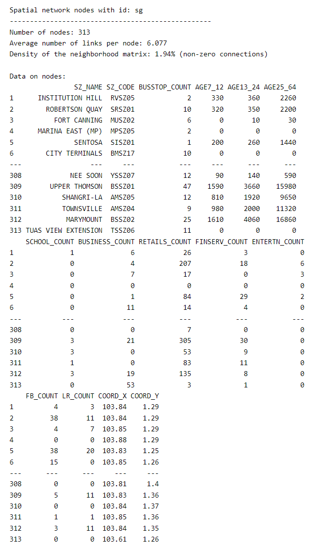
Creating spflow_network-class object
spflow_network-class object is an S4 class which holds information on origin-destination (OD) pairs. Each OD pair is composed of two nodes, each belonging to one network. All origin nodes must belonging to the same origin network should be contained in one spflow_network-class onject and likewise for the destination.
mpsz_net_pairs <- spflow_network_pair(
  id_orig_net = "sg",
  id_dest_net = "sg",
  pair_data = mpsz_flow,
  orig_key_column = "ORIGIN_SZ",
  dest_key_column = "DESTIN_SZ")

mpsz_net_pairs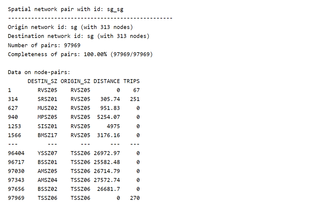
Creating sp_multi_network-class object
The sp_multi_network-class combines information on the nodes and the node-pairs and also ensures that both data sources are consistent. For example, if some of the origins in the sp_network_pair-class are not identified with the nodes in the sp_network_nodes-class an error will be raised.
mpsz_multi_net <- spflow_network_multi(mpsz_net,
                                       mpsz_net_pairs)
mpsz_multi_net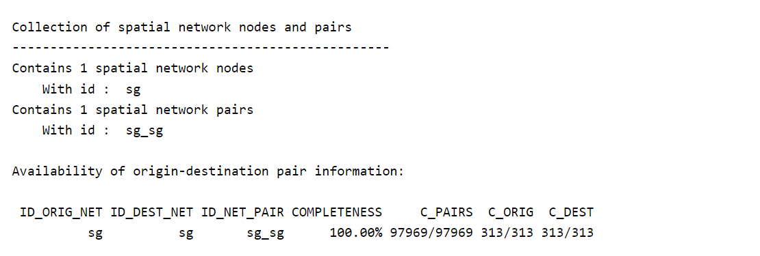
cor_formula <- log(1 + TRIPS)~
  BUSSTOP_COUNT +
  AGE7_12 +
  AGE13_24 +
  AGE25_64 +
  SCHOOL_COUNT +
  BUSINESS_COUNT +
  RETAILS_COUNT +
  FINSERV_COUNT +
  P_(log(DISTANCE +1))

cor_mat <- pair_cor(
  mpsz_multi_net,
  spflow_formula = cor_formula,
  add_lags_x = FALSE)

colnames(cor_mat) <- paste0(       #label the variables
  substr(
    colnames(cor_mat),1,3),"...")

cor_image(cor_mat) # to construct the correlation matrix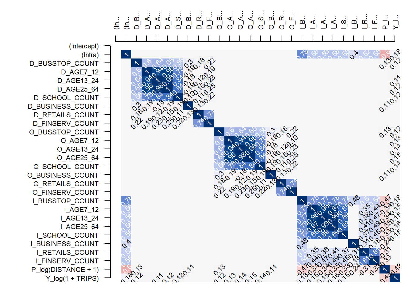
The Base Model
base_model <- sp_flow(
  spflow_formula = log(1 + TRIPS) ~
    O_(BUSSTOP_COUNT +
         AGE25_64) +
    D_(SCHOOL_COUNT +
         BUSINESS_COUNT +
         RETAILS_COUNT +
         FINSERV_COUNT) +
    P_(log(DISTANCE +1)),
  spflow_networks = mpsz_multi_net)

base_model
In the code chunk below, spflow_moran_plots() is used.
old_par <- par(mfrow = c(1.3),
               mar = c(2,2,2,2))
spflow_moran_plots(base_model)
par(old_par)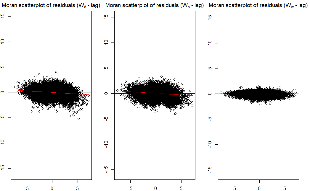
Next, pair_cor() can be used to inspect the relationship of the residual and the explanatory variables by using the code chunk below.
corr_residual <- pair_cor(base_model)
colnames(corr_residual) <- substr(colnames(corr_residual),1,3)
cor_image(corr_residual)
Working with Model Control
spflow_formula <- log(1+TRIPS)~
  O_(BUSSTOP_COUNT +
       AGE25_64) +
  D_(SCHOOL_COUNT +
       BUSINESS_COUNT +
       RETAILS_COUNT +
       FINSERV_COUNT) +
  P_(log(DISTANCE + 1))

model_control <- spflow_control(
  estimation_method = "mle",
  model = "model_8")

mle_model8 <- spflow(
  spflow_formula,
  spflow_networks = mpsz_multi_net,
  estimation_control = model_control)

mle_model8
old_par <- par(nfrow = c(1,3),
mar = c(2,2,2,2))
spflow_moran_plots(mle_model8)
par(old_par)