pacman::p_load(tmap, sf, tidyverse)In-Class Exercise 1- My First Date with Geospatial Data Analytics
1. Getting Started
1.1 Install and launching the R packages
The code chunk below load the following packages:
tmap: for thematic mappingsf: for geospatial data handlingtidyverse: for non-spatial data handling
1.2 Preparing the Flow Data
Create a folder called aspatial and save it in the data folder. Place the origin_destination_bus csv file into the aspatial folder.
1.2.1 Importing the OD data
Firstly, we will import the Passenger Volume by Origin Destination Bus Stops data set downloaded from LTA DataMall by using read_csv() of readr package.
odbus <- read.csv("data/aspatial/origin_destination_bus_202308.csv")A quick check of the odbus tibble data frame shows that the values in the ORIGIN_PT_CODE and DESTINATION_PT_CODE are numerical variables that are categorical in nature. The code chunk below transforms the ORIGIN_PT_CODE and DESTINATION_PT_CODE into factors, so that R treats them as a grouping variable.
odbus$ORIGIN_PT_CODE <-
  as.factor(odbus$ORIGIN_PT_CODE)

odbus$DESTINATION_PT_CODE<-
  as.factor(odbus$DESTINATION_PT_CODE)
1.2.2 Extracting the study data
For the purpose of this exercise, we will extract commuting flows on weekday and between 7 and 9 o’clock.
origin7_9 <- odbus %>%
  filter(DAY_TYPE == "WEEKDAY") %>%
  filter(TIME_PER_HOUR >= 7 &
           TIME_PER_HOUR <= 9) %>%
  group_by(ORIGIN_PT_CODE) %>%
  summarise(TRIPS = sum(TOTAL_TRIPS))
1.2.3 Importing geospatial data
Two geospatital data will be used in this exercise, they are:
1. Bus stop Location
busstop <- st_read(dsn = "data/geospatial",
                   layer = "BusStop") %>%
  st_transform(crs=3414)
Reading layer `BusStop' from data source
`C:\Users\Dabbie Neo\Desktop\Geospatial_Analytics\dneoo\ISSS624\In-class_Ex\In-class_Ex01\data\geospatial'
using driver `ESRI Shapefile'
Simple feature collection with 5161 features and 3 fields
Geometry type: POINT
Dimension: XY
Bounding box: xmin: 3970.122 ymin: 26482.1 xmax: 48284.56 ymax: 52983.82
Projected CRS: SVY212. Planning Subzone area
mpsz <- st_read(dsn = "data/geospatial",
                layer = "MPSZ-2019") %>%
  st_transform(crs =3414)
Reading layer `MPSZ-2019' from data source
`C:\Users\Dabbie Neo\Desktop\Geospatial_Analytics\dneoo\ISSS624\In-class_Ex\In-class_Ex01\data\geospatial'
using driver `ESRI Shapefile'
Simple feature collection with 332 features and 6 fields
Geometry type: MULTIPOLYGON
Dimension: XY
Bounding box: xmin: 103.6057 ymin: 1.158699 xmax: 104.0885 ymax: 1.470775
Geodetic CRS: WGS 84mpszSimple feature collection with 332 features and 6 fields
Geometry type: MULTIPOLYGON
Dimension: XY
Bounding box: xmin: 2667.538 ymin: 15748.72 xmax: 56396.44 ymax: 50256.33
Projected CRS: SVY21 / Singapore TM
First 10 features:
SUBZONE_N SUBZONE_C PLN_AREA_N PLN_AREA_C REGION_N
1 MARINA EAST MESZ01 MARINA EAST ME CENTRAL REGION
2 INSTITUTION HILL RVSZ05 RIVER VALLEY RV CENTRAL REGION
3 ROBERTSON QUAY SRSZ01 SINGAPORE RIVER SR CENTRAL REGION
4 JURONG ISLAND AND BUKOM WISZ01 WESTERN ISLANDS WI WEST REGION
5 FORT CANNING MUSZ02 MUSEUM MU CENTRAL REGION
6 MARINA EAST (MP) MPSZ05 MARINE PARADE MP CENTRAL REGION
7 SUDONG WISZ03 WESTERN ISLANDS WI WEST REGION
8 SEMAKAU WISZ02 WESTERN ISLANDS WI WEST REGION
9 SOUTHERN GROUP SISZ02 SOUTHERN ISLANDS SI CENTRAL REGION
10 SENTOSA SISZ01 SOUTHERN ISLANDS SI CENTRAL REGION
REGION_C geometry
1 CR MULTIPOLYGON (((33222.98 29...
2 CR MULTIPOLYGON (((28481.45 30...
3 CR MULTIPOLYGON (((28087.34 30...
4 WR MULTIPOLYGON (((14557.7 304...
5 CR MULTIPOLYGON (((29542.53 31...
6 CR MULTIPOLYGON (((35279.55 30...
7 WR MULTIPOLYGON (((15772.59 21...
8 WR MULTIPOLYGON (((19843.41 21...
9 CR MULTIPOLYGON (((30870.53 22...
10 CR MULTIPOLYGON (((26879.04 26...st_read()function of a sf package is used to import the shapefile into R as sf data frame.
busstop_mpsz <- st_intersection(busstop, mpsz) %>%
  select(BUS_STOP_N, SUBZONE_C) %>%
  st_drop_geometry()
origin_SZ <- left_join(origin7_9 , busstop_mpsz,
by = c("ORIGIN_PT_CODE" = "BUS_STOP_N")) %>%
rename(ORIGIN_BS = ORIGIN_PT_CODE,
ORIGIN_SZ = SUBZONE_C) %>%
group_by(ORIGIN_SZ) %>%
summarise(TOT_TRIPS = sum(TRIPS))duplicate <- origin_SZ %>%
group_by_all() %>%
filter(n()>1) %>%
ungroup()origin_data <- unique(origin_SZ)origintrip_SZ <- left_join(mpsz,
origin_SZ,
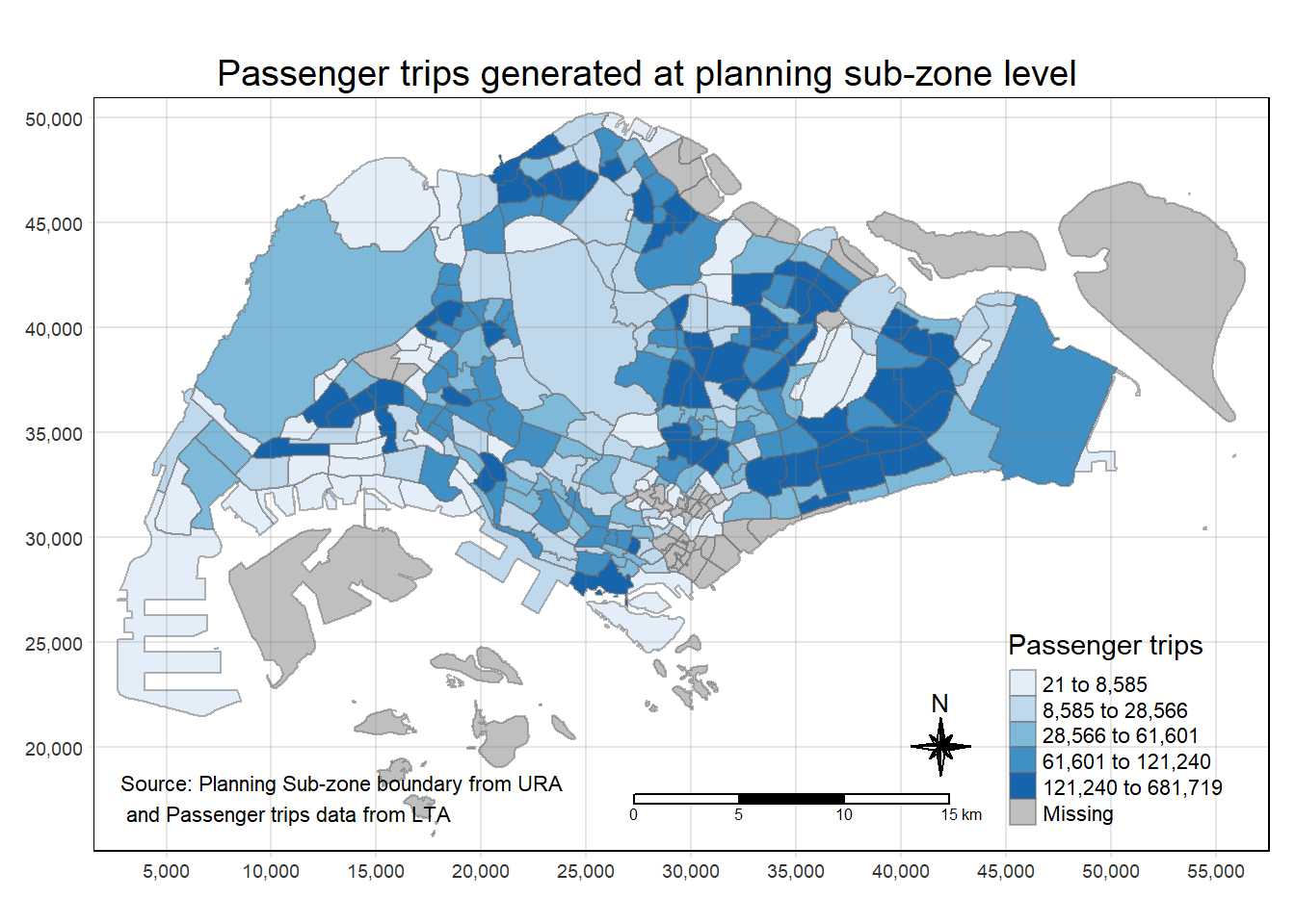
by = c("SUBZONE_C" = "ORIGIN_SZ"))tmap_mode("plot")
tm_shape(origintrip_SZ)+
tm_fill("TOT_TRIPS",
style = "quantile",
palette = "Blues",
title = "Passenger trips") +
tm_layout(main.title = "Passenger trips generated at planning sub-zone level",
main.title.position = "center",
main.title.size = 1.2,
legend.height = 0.45,
legend.width = 0.35,
frame = TRUE) +
tm_borders(alpha = 0.5) +
tm_compass(type="8star", size = 2) +
tm_scale_bar() +
tm_grid(alpha =0.2) +
tm_credits("Source: Planning Sub-zone boundary from URA\n and Passenger trips data from LTA",
position = c("left", "bottom"))